In a humid environment such as in Okinawa during the Baiu period, convective cells whose echo-top height was quite low and those in a stratiform rain zone were observed. For clarifying the distributions of precipitation particles in these convective cells, we performed observations on Okinawa Island during the Baiu period using a C-band polarimetric radar and a disdrometer.
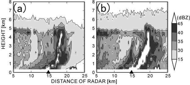
We analyzed polarimetric variables and rain drop size distribution (DSD) in convective cells associated with the Baiu frontal rainband on June 10, 2006 using polarimetric radar and disdrometer data. Two convective cells were selected for the analysis. One was embedded in a stratiform rain zone (Fig. 1a) and the other existed in a convective rain zone (Fig. 1b) associated with rainbands. Both convective cells had low echo-top heights (of 30 dBZe) below the height of 6 km, and exhibited intense reflectivity in their convective cores. By analyzing the polarimetric variables, it was determined that a large number of small raindrops contributed to the intense reflectivity below the height of 3.5 km in the former case. This fact was supported by DSD observations, which showed the large contribution of small raindrops (1 to 2 mm in diameter) to the strong rainfall intensity on the ground. Some large raindrops contributed to the intense reflectivity in the latter case. This fact was also supported by DSD observations, which showed the large contribution of large raindrops (exceeding 3 mm in diameter) to the strong rainfall intensity on the ground. From these results, the distribution of precipitation particles in each convective cell was expressed schematically in Fig. 2.
To confirm the generality of this result, 31 convective cells embedded in the stratiform rain zone and 29 cells in the convective rain zone were analyzed using polarimetric variables. A large number of small raindrops contributed to the intense reflectivity in convective cells embedded in the stratiform rain zone, and large raindrops contributed to the reflectivity in the convective rain zone below the height of 3.5 km. These characteristics were the same as those of the two convective cells mentioned above. Thus, we revealed the two types of distributions of precipitation particles in convective cells associated with the Baiu frontal rainband on June 10, 2006; the predominance of small raindrops in the convective cell embedded in the stratiform rain zone, and the existence of large raindrops in the convective rain zone.
Fig. 1: Vertical distribution of radar reflectivity in RHI of the convective cell embedded in the stratiform rain zone (a), and that in the convective rain zone (b). The symbol ▲ denotes the position of the disdrometer observation site.
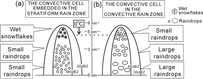
Fig. 2: Schematic distribution of precipitation particles in the convective cell embedded in the stratiform rain zone (a), and that in the convective rain zone (b).
This study revealed the structure of "precipitation cell lines (PCLs)" oblique to the Baiu front generated around the Southwest Islands of Japan on June 10, 2006, using data obtained from two X-band Doppler radars located at Shimoji and Tarama Islands.
PCLs appeared every several tens of kilometers in the heavy rainfall area along the Baiu front, extending from west-southwest (WSW) to east-northeast (ENE) for 300 km (Fig. 3). These PCLs consisted of several precipitation cells aligned from south-southwest (SSW) to north-northeast (NNE). The length of the PCLs ranged from 20 to 40 km, and the alignment of the PCLs was parallel to the vertical wind shear between 0.5 and 3 km in altitude. Precipitation cells were generated in the southern part of PCLs, where a large low-level convergence area existed. They moved northeastward corresponding to the horizontal wind velocity at the height of 3 km, and decayed in the northern part of the PCLs, where a large low-level divergence area existed (Fig. 4). The cells in the southern part of the PCLs were in the developing stage in their life-cycle, those in the central part were mature, and those in the northern part were in the decaying stage (Fig. 5).
New cells constructing PCLs were generated at the rear of the pre-existing cells that propagated northeastward. This structure represented the characteristics of the "back-building" line-shaped precipitation systems. However, the downdraft of the pre-existing cell was weak, and the low-level southward flow from the northern cells was not observed by dual-Doppler analyses (Fig. 5). The fact that pre-existing cells did not affected on the generation of new cells should be attributed to the lack of evaporation cooling, due to the high humid field in the lower troposphere around the Baiu front. Further, convectively neutral stratification appeared in the northern part of the PCLs. Therefore, the new cells developed only in the southern part of the PCLs, where a low-level convergence existed along the Baiu front. The length of the PCLs corresponded to the product of the life span and speed of each cell relative to the PCL. Thus, using only observation data, this study revealed that PCLs oblique to the Baiu front were the "back-building" line-shaped precipitation systems that occurred in the high humid field in the lower troposphere.
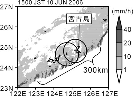
Fig. 3: Rainfall intensity distributions observed by the JMA radar at 1500 JST on June 10, 2006. The ranges of the Doppler radars installed at Shimoji and Tarama Islands are indicated by circles.
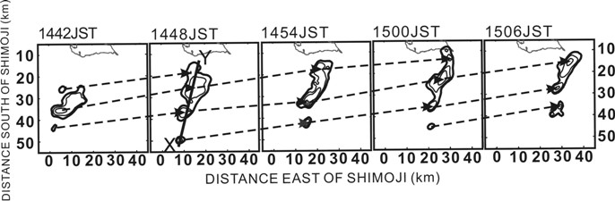
Fig. 4: Reflectivity distributions at the height of 2 km observed by Doppler radars at 6-min intervals from 1442 to 1506 JST on June 10, 2006. Only the precipitation area related to a PCL is shown. The reflectivity is contoured at 2-dBZe intervals from 32 dBZe. The arrows indicate the propagation of each precipitation cell.
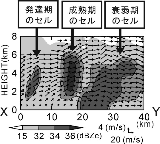
Fig. 5: Vertical cross section of the distribution reflectivity (shades) and horizontal and vertical wind vectors (arrows) at 1448 JST on June 10, 2006 along the X-Y line of Fig. 4.
Tornadoes and waterspouts are a violently rotating air below a convective cloud. They are called ``tatsumaki'' in Japan. In Japan, 20.5 tornadoes and 4.5 waterspouts occur on average and about 20% of tornadoes occur in association with typhoons.
Even through a typhoon center is located in the far distance, a disaster due to a strong wind is occasionally caused by a ``tatsumaki.'' When Typhoon 0613 (T0613) moved northward off the west of Kyushu, a severe disaster was caused by an intense tatsumaki along the east coast of Kyushu. The tatsumaki occurred when typhoon rainbands moved northward along the east coast. Two simulations with different horizontal resolutions were performed using the Cloud Resolving Storm Simulator (CReSS) Ver.2.2 in the present study. The experiment with a horizontal resolution of 500 m successfully simulated not only the overall structure and movement of T0613 but also a detailed structure of the typhoon rainbands. The other experiment with a resolution of 75 m simulated that a tatsumaki formed in convective clouds. The result showed that the outermost rainband was composed of suprecells which involve a meso-cyclone. Tatsumakis formed within the supercells.
A detailed structure of the supercell which produced a tatsumaki was simulated (Fig. 6). The supercell extends the north-south direction with a horizontal length of 20 km. Intense rain occurred in the southern part of the supercell with a very sharp hook-shaped structure at the southernmost part. The tatsumaki is formed in the hook-shaped structure which is indicated by the circle in Fig. 6. A weak rain is present in the northern part of the cell. A close view of the southern part of the supercell (Fig. 7) shows that the tatsumaki forms inside of the hook. The horizontal scale of the simulated tatsumaki is about 300 m, which is the almost same scale with the observed tatsumaki. The experiment of 75-m resolution successfully simulates the tatsumaki within the supercell. The maximum vorticity of the tatsumaki is 0.9 s-1 and pressure perturbation at the center is -27 hPa. The pressure field and the velocity field are in the cyclostrophic balance in a high accuracy. This is a most significant characteristic of the tatsumaki.
The wind velocity around the tatsumaki is very large which resulted in the severe disaster in Nobeoka City. The horizontal wind speed of the simulated tatsumaki is larger than 70 m s-1 on the east side of the tatsumaki while it is weak in the west side (Fig. 8). This asymmetry of horizontal wind speed well corresponds to the asymmetry of the damage distribution due to the tatsumaki. The damage is significant on the right-hand side of the pass of the tatsumaki while it is small on the left-hand side with the northward movement of the tatsumaki.
Another simulation experiment with a horizontal resolution of 75 m was performed within a much larger domain using the Earth Simulator. A preliminary result shows many tatsumakis were simulated along the typhoon rainbands. Most tatsumakis form along the northernmost (outermost) rainband. This is consistent with that the outermost rainband is composed of supercells in the experiment of 500-m resolution.
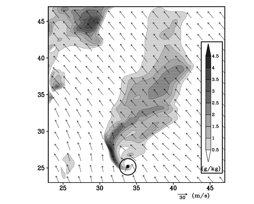
Fig. 6: Supercell at a height of 200 m at 0500 UTC September 17, 2007 obtained form 75-m resolution simulation. Gray levels are mixing ratio of rain (g kg-1) and arrows are horizontal velocity. The circle indicates the tatsumaki developed in the supercell.
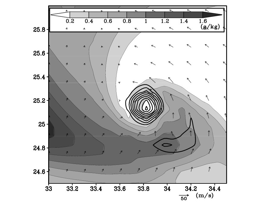
Fig. 7: Enlarged view of the southernmost part of the supercell indicated by the circle in Fig. 6. Gray levels are mixing ratio of rain (g kg-1), contours are vertical voriticity from 0.1 s-1 every 0.1 s-1, and arrows are horizontal velocity.
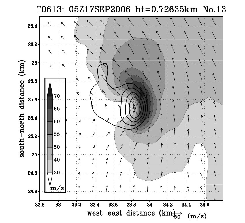
Fig. 8: Horizontal distribution of wind speed (gray levels; m s -1) at a height of 0.73 km at 0500 UTC September 17, 2006.
Strong winds and heavy rainfall associated with typhoons cause large damage. Highly accurate typhoon forecasts are required to estimate the damage region and non-life insurance premiums. In order to forecast extreme phenomena, it is necessary to use a high-resolution numerical model that resolves spiral rainbands of a typhoon. In this study, we simulated 10 typhoons that caused large damage in Japan, using the Cloud Resolving Storm Simulator (CReSS) and evaluated the results.
Figure 9 shows the observed best track and the results of a 48-h numerical simulation for typhoon Songda (T0418). The simulated track, landfall point on Kyushu Island, and acceleration of the typhoon after landfall, are reproduced well. Although the central pressure error at the initial time is about 20 hPa, it decreased until six hours from the start of the simulation. During the landfall on Kyushu Island, the minimum pressure near the center of the typhoon is 945 hPa and the error is only 1 hPa. The maximum wind speed of over 35 m s-1 and the heavy rainfall around Kyusyu are also reproduced well. Thus, the track and intensity of typhoon Songda were successfully simulated using the CReSS.
Next, quantitative validations were performed for all 10 cases. Figure 10 shows a histogram of the rainfall over 20 mm h-1. The CReSS (horizontal grid resolution; dx = 2.5 km) reproduces this heavy rainfall well compared with that reproduced by the Regional Spectral Model (RSM: dx = 20 km). The wind gust is a key parameter for wind disasters. Figure 11 shows a scatter plot of the maximum wind speed observed at meteorological stations and the estimated maximum wind speed calculated from the product of the simulated wind speed and statistical gust ratio in the same grid in the CReSS simulations. The correlation between the simulated and observed wind speeds is very high, 0.83. Therefore, we can consider that the CReSS reproduces the typhoons quite well.
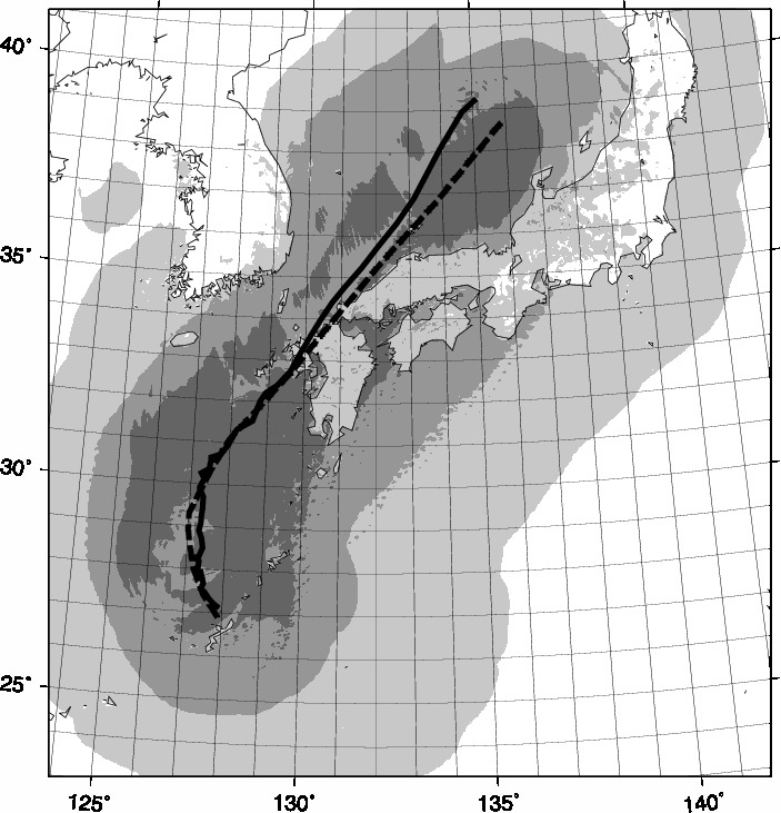
Fig. 9: Best track (broken) and simulated track (solid) of the typhoon Songda. The shaded areas show strong wind regions: 15, 25, and 35 m s -1, respectively.
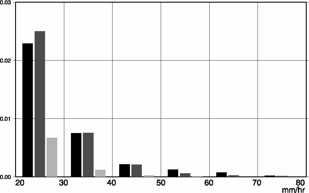
Fig. 10: Histogram of rainfall above 20 mm h-1 by observation (black), CReSS (dark grey), and RSM (light grey).
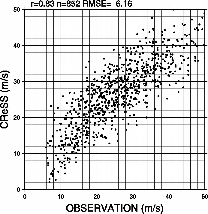
Fig. 11: Scatter plot of the maximum wind speed observed at meteorological stations, and the estimated maximum wind speed calculated from the simulation results.
There is a large uncertainty about the large-scale condensation processes that prescribe the development of clouds in the general circulation model (GSM). The large-scale condensation processes prescribe the amount of condensation (cloud water/ice amounts) and cloud fraction in each grid, as a result of the prescribed probability density function (PDF) that is assumed for the average value of total water. In this study, we show a PDF for total water using daily simulation results from the Cloud Resolving Strom Simulator (CReSS) for the area around Japan from December 29, 2004 to December 16, 2005. The total number of simulations was 303. The horizontal and vertical grid resolutions of the simulation were 5 and 0.5 km, respectively. Data of every hour from the start of the simulation were used for the PDF analysis. Mixing ratio of total water, which was the sum of that of water vapor, cloud water, rain, cloud ice, snow, and graupel, was averaged for the horizontal scale of about 280×280 km2, which supposed a horizontal grid resolution of T42-GCM. The PDF of total water was calculated in each bin (every 0.1 g kg-1) of averaged mixing ratio of total water for each grid, and their frequency in each bin was accumulated. We show the standard deviation and skewness for each bin of averaged mixing ratio of total water for the PDF analysis.
Figure 12 shows the standard deviation and skewness profiles of grid-averaged mixing ratio of total water in a GCM grid scale. The standard deviation and skewness are 1.2 g kg-1 and 0.2, respectively, between 5 and 15 g kg-1 of GCM-grid averaged total water. Although each frequency distribution is different, e.g., there are peaky, double peak, and broad shaped distributions, the PDF shape should be attributed to the Gaussian distribution, if we suppose the bulk PDF of total water. This results show that the Gaussian distribution should be applied to the PDF in the large-scale condensation process.
The standard deviation is small for small mixing ratio of total water less than 5 g kg-1. This should be attributed to the effect of the lower limit of mixing ratio. The skewness has large positive values in this case. For small mixing ratio of total water, temperature should be quite low. Thus, it should be considered that the PDF expands to large mixing ratio due to the existence of ice particles, which has a small fall velocity. On the other hand, the standard deviation is also small, and the skewness has small negative values for large mixing ratio of total water larger than 15 g kg-1. This should be attributed to the effect of the upper limit of relative humidity. In this case, condensates should be liquid (rain), and they are removed from the grid quickly because of its large falling velocity. As a result, the PDF reduces on the larger side of mixing ratio.
These features are not varied for latitude and layers (height). However, those over the ocean are different from those over land, and a profile of standard deviation in winter differs from those in other seasons. More analysis is required using cloud resolving models to understand the PDF well, and to improve the large-scale condensation processes in the GCM.
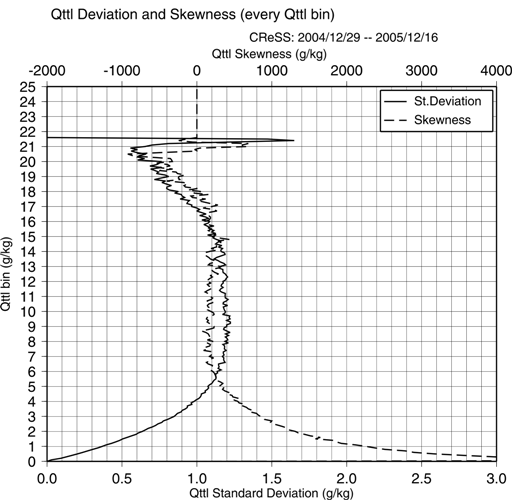
Fig. 12: Standard deviation (solid line) and skewness (broken line) profiles of mixing ratio of total water for the grid averaged one in a GCM grid scale. Skewness a thousandfold times is shown.
We investigated the characteristics of precipitation systems for heavy rainfall in Bangladesh (88.05-92.74 deg. E, 20.67-26.63 deg. N), which is influenced by the Asian monsoon system. Precise understanding of the distribution and characteristics of precipitation systems is useful for disaster prevention and water management in an agriculture-dependent country like Bangladesh.
Six years of S-band weather radar data from 2000, obtained by the Bangladesh Meteorological Department, were used to reveal the characteristics of precipitation systems. Precipitation systems with a lifetime longer than three hours and a dimension larger than 100 km (long axis) were analyzed. We identified the shape, horizontal scale, propagation speed, and lifetime as the characteristics of precipitation systems. The precipitation systems were classified into Arc, Line, and Scattered types, according to their shape. The systems were divided according to the length of their long axis into small scale (SS, from 100 to 200 km), medium scale (MS, 200 to 300 km), and large scale (LS, larger than 300 km). Based on the propagation speed, the systems were divided into stationary (less than 2 m s-1), slow moving (2 to 7 m s-1), and fast moving (larger than 7 m s-1 ). The approximate lifetime of the systems was calculated from available scans.
The frequencies of the Arc-, Line-, and Scattered-type systems were determined to be 230 (29%), 117 (15%), and 442 (56%), respectively, from April to September during the analysis years. For the Arc-, Line-, and Scattered-type systems, the averaged horizontal scales were about 185, 184, and 268 km; propagation speeds were 11.0, 7.1, and 5.8 m s-1 ; and approximately lifetimes were 4.3, 4.0, and 4.8 h, respectively. The Scattered-type system dominated during the monsoon period (June, July, August, and September), while the Arc-type dominated in the pre-monsoon period (April and May). The Line-type system had an almost equal frequency of occurrence in both periods. Systems that developed in the monsoon period were long and stationary or slow moving, whereas systems in the pre-monsoon period were small and fast moving. Systems in the pre-monsoon period propagated southeastward, whereas those in the monsoon season propagated northwestward, northeastward, and southeastward (Fig. 13).
This analysis discloses that the population of precipitation systems is high in the southern, eastern, and northern part of Bangladesh (Fig. 14). Of the total of 442 Scattered-type systems, 244 covered a wide area, which was beyond radar range, and moved slowly. We called these systems the Scattered-type systems having wide areal coverage (SWAC). This analysis revealed that about 97% of the SWAC developed during the monsoon period and it made a huge contribution to monsoon rainfall in this region.
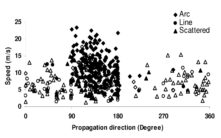
Fig. 13: Propagation speed and direction of different types of systems. The precipitation systems whose propagation speed was not observed and the SWAC are not shown. Solid and open symbols represent the systems that developed in the pre-monsoon and monsoon periods, respectively.
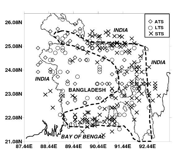
Fig. 14: Spatial distribution of different types of systems that developed in and around Bangladesh during the monsoon period. The dashed line represents the wet region presented by Islam and Uyeda (2007). The SWACs are not shown.